
Your embedding model doesn’t understand your data
INTERNALS.md #3 · It never did. Here’s what it actually does, and why that matters for every RAG system you’ll ever build.

Here’s a bug that doesn’t show up in your logs.
You ship a RAG system. Users ask questions about internal data: support tickets, product docs, sales notes. Cosine similarity scores come back at 0.74, 0.81, 0.78. The LLM generates a confident, fluent answer.
While the resulting answers aren’t always obviously broken, they fail in a specific, repeatable pattern.
Someone asks about “pipeline” and gets sales documents when they meant data infrastructure.
Someone asks about “incident” and gets both engineering postmortems and customer support tickets, randomly.
Someone asks about “ARR attainment” and gets a document about spreadsheet formulas.
You tune the prompts. You adjust chunk sizes. The results are still wrong.
Prompt engineering and chunking strategies fail here because the root cause lies in how the foundational vector space is created.
A note before we start. This post assumes you’ve shipped or worked on a RAG system and have firsthand experience with it underperforming on domain-specific queries. If you need a foundation first, this primer is a solid 10 minutes. You’ll get more from this post with that context.
The Blueprint:
The Illusion: Why your embedding model is a map of the internet, not an understanding machine.
The Geometry: How high-dimensional space pathology compresses your similarity scores.
The Failure Modes: How to diagnose and fix the 4 silent bugs killing domain retrieval (including Hubness and Concept Collision).
The Playbook: A 3-step engineering roadmap to evaluate, adapt, and fine-tune your space.
What you think is happening
Most engineers picture an embedding model as a kind of understanding machine.
You feed it text. It reads the text, grasps the meaning, and produces a number that represents that meaning.
Two pieces of text with similar meanings get similar numbers. You compare numbers. You find meaning.
This mental model feels right. It explains why “cat” and “feline” end up close together. It explains why the system works at all.
But this mental model is wrong, and that’s exactly why several production RAG pipelines fail.
Maps, not minds
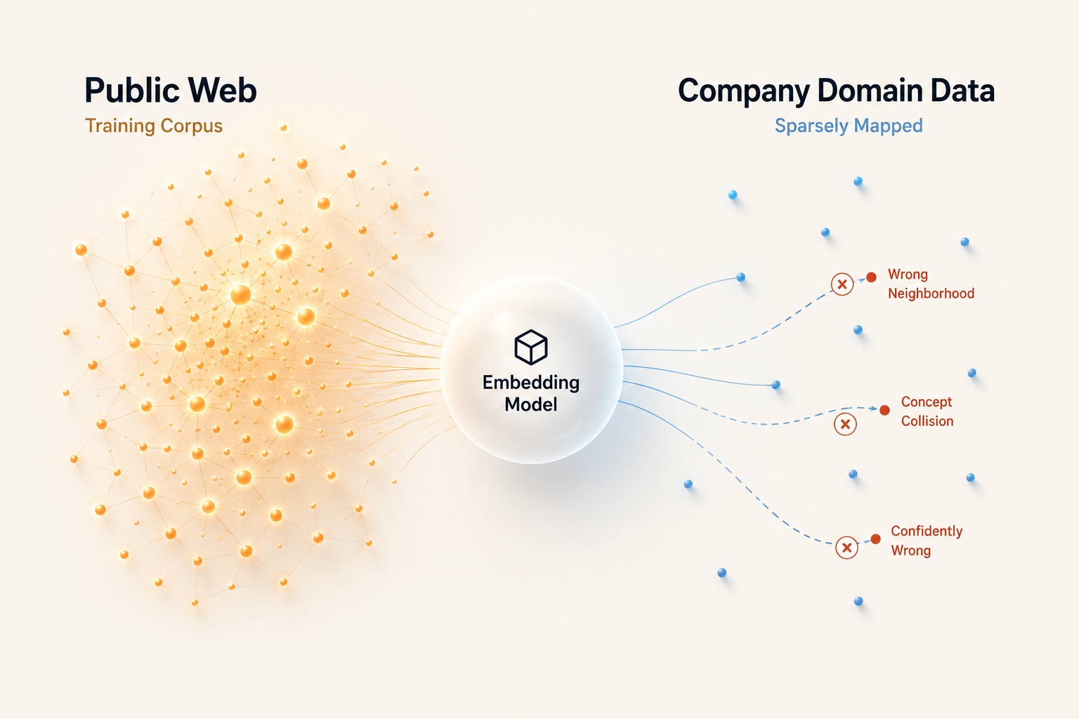
An embedding model doesn’t understand anything. They possess zero semantic comprehension. They strictly operate as coordinate systems - a map of language drawn by learning how words and phrases appeared in the internet.
Every piece of text you feed it gets assigned a location on that map. Texts that appeared together constantly, in the same articles, answering the same kinds of questions, end up near each other. The model never gets to redraw the map when it sees your internal data. It just projects everything onto the existing one, using whatever surface patterns and statistical echoes it recognizes.
The crucial part: the map was drawn by reading the internet.
Billions of web pages, Wikipedia articles, Reddit threads, news posts, academic papers. It’s a dense, detailed map of how language is used on the open web. This is why it works well for general questions. “Cat” and “feline” appeared near each other constantly. “Paris” and “capital of France” showed up together in thousands of articles.
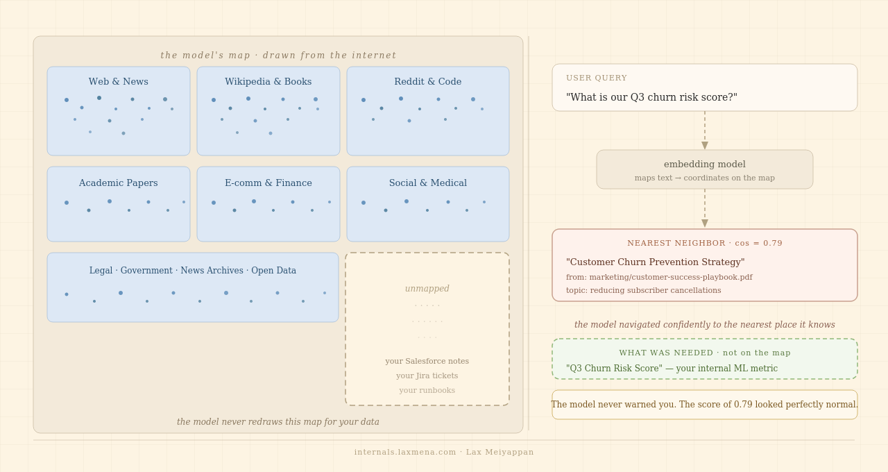
But your company’s specific use of “pipeline”, “incident”, “P0”, or “ARR attainment”? Those meanings were never on the original map. The model does the only thing it can: it finds the nearest coordinates it does have. It always returns something. There is no “I don’t know”.
Here is the part that makes this dangerous: the model never warns you. It returns a confident-looking coordinate and a plausible similarity score regardless of whether your data falls within the model’s training distribution or unmapped domain. A 0.79 similarity score looks identical for both a perfectly relevant retrieval and a catastrophic silent failure.
The cosine score only tells you distance on the map. It doesn’t tell you whether the map covers your territory.
↓ Internals
The formal name for this is the distributional hypothesis, stated by linguist J.R. Firth in 1957: “you shall know a word by the company it keeps”. Modern embedding models are this hypothesis at scale, with a neural network as the function approximator.
The model learns: text → a point in ℝⁿ (768 dimensions for BERT-base, 1536 for OpenAI’s text-embedding-3-small). Positions are determined entirely by co-occurrence patterns in the training corpus. A concept that appeared with insufficient frequency or in the wrong context distribution gets placed at unreliable coordinates. Not missing, just wrong.
The map has a geometry problem
Even when you’re asking about something the model did learn from the internet, the similarity scores can mislead you. And the reason has nothing to do with meaning.
When you compare two embeddings, you’re computing the angle between them. Small angle = similar. Large angle = different. This is called cosine similarity.
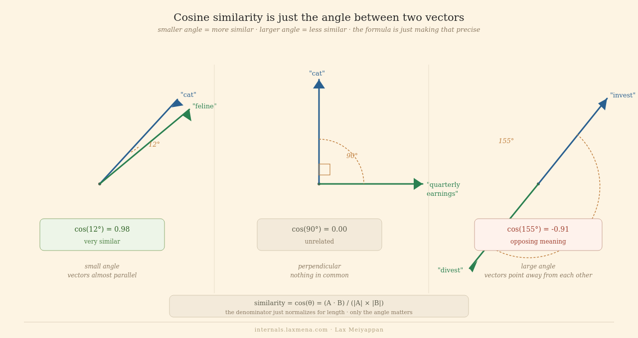
In 2D, this works well. Arrows can point in many directions. Two random arrows have a wide variety of angles, so you can clearly tell similar from different.
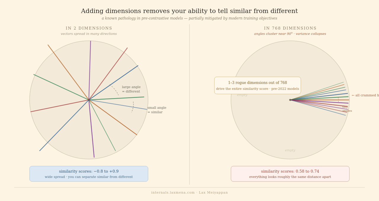
Now go to 768 dimensions. Something counterintuitive happens.
In raw high-dimensional spaces, the expected angle between random vectors concentrates near 90°. Modern contrastive objectives (the training method used by OpenAI, Cohere, BGE, and similar models) push useful variance into the tails and partially fix this. But when your data distribution differs from what the model was trained on, the collapse returns in practice: your domain queries end up in a poorly-calibrated corner of the space, and the scores stop being informative.
There’s a second problem on top of this.
Research from 2021 (Timkey & van Schijndel) measured exactly which dimensions drive cosine similarity scores in pre-contrastive BERT-style models. Their finding: just 1 to 3 dimensions out of 768 dominate the entire similarity calculation. The other 765 barely matter.
These are dimensions with unusually high variance that spread wide across the corpus. Because cosine similarity is an angle calculation, whatever dimensions spread widest have the most influence. The good news: simple post-processing (subtracting the mean, standardizing) largely mitigates rogue dimensions, and modern contrastive models have improved significantly. The caveat: when you’re running a general model on out-of-distribution domain data, these geometric pathologies re-emerge in subtler forms. You won’t know unless you measure.
↓ Internals
This is called anisotropy. Pre-trained transformer models produce spaces where vectors cluster into a narrow cone rather than spreading evenly. When you compute cosine similarity in that cone, angular distances compress. Everything looks vaguely similar.
You can verify this on any model. Compute cosine similarity between 1,000 random document pairs from your corpus and plot the distribution. Standard deviation below 0.1 means a compressed space. A well-calibrated contrastive model shows variance above 0.2 on genuinely diverse documents.
The geometric fix is contrastive training, using (query, positive, hard negative) triplets that push vectors apart more uniformly. This is what separates modern embedding models from older BERT-style ones.
Your data is a different country
Now put both problems together.
The map was drawn from the internet. The map’s geometry loses resolution in high dimensions. And your users are querying for domain-specific contexts that never existed in the base model’s training corpus.
In practice: your model confidently navigates general topics. Common business language, standard industry terms, broad concepts. The map is detailed there. But when your users ask about your company’s specific vocabulary, the model has no coordinates for those meanings. It falls back to surface patterns: which words the document contains, what those words meant on the internet.
A 2024 study tested seven state-of-the-art embedding models on financial domain text: SEC filings, earnings calls, analyst reports. Every model performed significantly worse on domain text than on the general benchmark. More striking: a model’s general benchmark score had almost no correlation with its domain performance. The rankings reshuffled completely.
The general benchmark tells you how well the map covers the internet. It says nothing about your territory.
↓ Internals
Domain failure isn’t just missing vocabulary. Most domain terms exist somewhere in the training corpus. Words like “ARR”, “churn”, and “pipeline” all appear in web text. The problem is the context distribution.
The word “Churn” in training data appears near “customer attrition”, “SaaS metrics”, “subscription”. In your network operations runbook, it appears near “packet loss”, “network degradation”. Same word, completely different neighborhood. The model maps it to web-scale coordinates. Your users’ queries navigate to the wrong neighborhood.
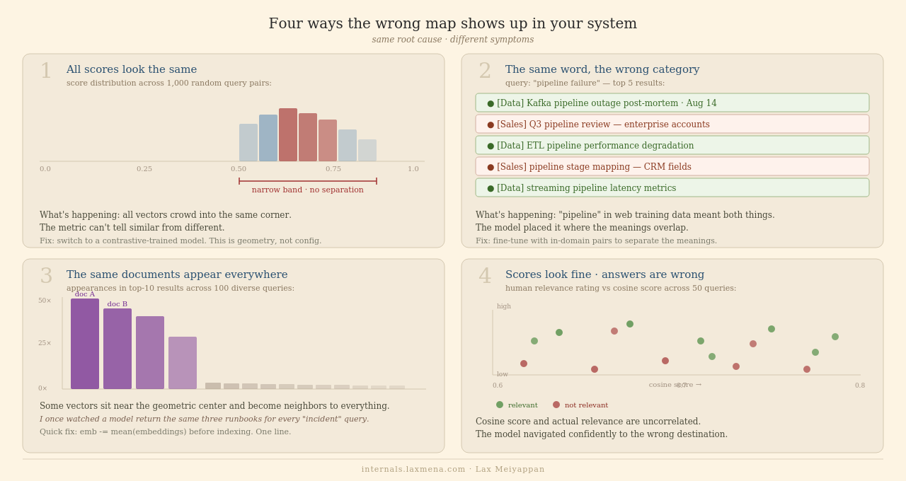
Four ways the wrong map shows up
These failure patterns look different on the surface. Underneath, they’re all the same problem.
1. All your similarity scores look the same
You query for something very specific. You query for something very general. The scores come back in the same narrow range regardless (say, 0.62 to 0.79) and don’t separate relevant from irrelevant.
What’s happening: your embedding space is compressed. All vectors crowd into the same corner. The metric can’t discriminate between meaningfully similar and meaningfully different.
Diagnostic: compute cosine similarity on 1,000 random document pairs. Standard deviation below 0.1 = compressed space.
Fix: switch to a model trained with contrastive objectives. This is a geometry problem. A configuration change won’t fix it.
↓ Internals: Vector Database is Just the Index
A common point of confusion for engineers building RAG stacks is separating the embedding model from the vector database (OpenSearch, Pinecone, pgvector, etc).
Think of your vector database as a high-performance book shelf. Its only job is to index, store, and look up coordinates as fast as possible using approximate nearest neighbor (ANN) algorithms like HNSW or IVF-PQ. It doesn’t generate the coordinates, and it doesn’t judge their semantic quality.
If your embedding model suffers from anisotropy, you are feeding the book shelf broken coordinates. You can tune your database’s ef_search parameters, payload indexes, or distance metrics all day, but you are ultimately just optimizing how fast the system retrieves nearby noise. The database is calculating the math perfectly; it’s the underlying geometry that is wrong.
2. The same word retrieves documents from the wrong category
“Pipeline” returns sales content when the user asked about data infrastructure. “Incident” mixes engineering postmortems/CoE’s with support tickets. Domain terms with one specific meaning in your organization keep returning documents from a different context.
What’s happening: concept collision. The model placed these terms at their web-scale coordinates, where they overlap multiple meanings. Your organization uses them narrowly; the training data used them broadly.
Diagnostic: for your five most domain-specific terms, manually inspect the top 10 retrieved documents. If a single-meaning term consistently returns two or more semantic categories, you have concept collision.
Fix: fine-tuning with pairs from your corpus. The training process will encounter these collision cases naturally and learn to separate them.
3. The same few documents appear in every result set
Across many different queries, five or ten documents keep showing up in your results. Not always obviously relevant. I once watched a model return the same three runbooks for every “incident” query. Scores looked great, all above 0.75. Turned out those runbooks were long, covered every keyword, and sat geometrically near the center of the cluster. Classic hub. One line of code fixed half the pain.
What’s happening: hubness. In high-dimensional compressed spaces, some vectors land near the geometric center of the distribution. These documents become close neighbors to almost everything. Not because they’re relevant, but because of where they sit geometrically.
Diagnostic: log which document IDs appear in top-10 results across 100 diverse queries. A small number appearing more than 20 times is a hub problem.
Quick fix:
embeddings -= embeddings.mean(axis=0) before indexing. Pushes hubs away from the center. Often produces immediate improvement.
Proper fix: switch to or fine-tune a model with better geometry.
4. Scores look fine but answers are wrong
Cosine scores are in a reasonable range. The LLM generates coherent text. But the answers are consistently, subtly wrong in ways no automated metric catches.
This is the hardest one to diagnose because everything in your pipeline looks healthy.
What’s happening: the model navigated confidently to the nearest coordinates it knows, which aren’t where you needed to go. The score is high because these really are the nearest neighbors on the map. They’re just neighbors on the wrong map.
Diagnostic: build 50 to 100 (query, relevant document, irrelevant document) triplets, manually curated. Measure NDCG@10. Below 0.5 on domain queries is a clear signal.
Fix: domain adaptation. Fine-tuning, or switching to a purpose-built model for your vertical.
↓ Internals: The Telemetry of a Blind Spot
When your embedding model drops the LLM into an unmapped “blank space” on the map, the LLM is forced to rely on its own pre-trained web priors to bridge the gap. This is the exact failure mode that RAGAS isolates.
While your vector database registers a confident 0.79 cosine similarity score, RAGAS measures Faithfulness (checking if the generated response is strictly inferable only from the retrieved text). If your embedding space is suffering from a massive domain shift, your cosine scores stay high, but your Ragas Faithfulness scores drop to zero - proving that a high similarity score on a broken map is just a measurement of nearby noise.
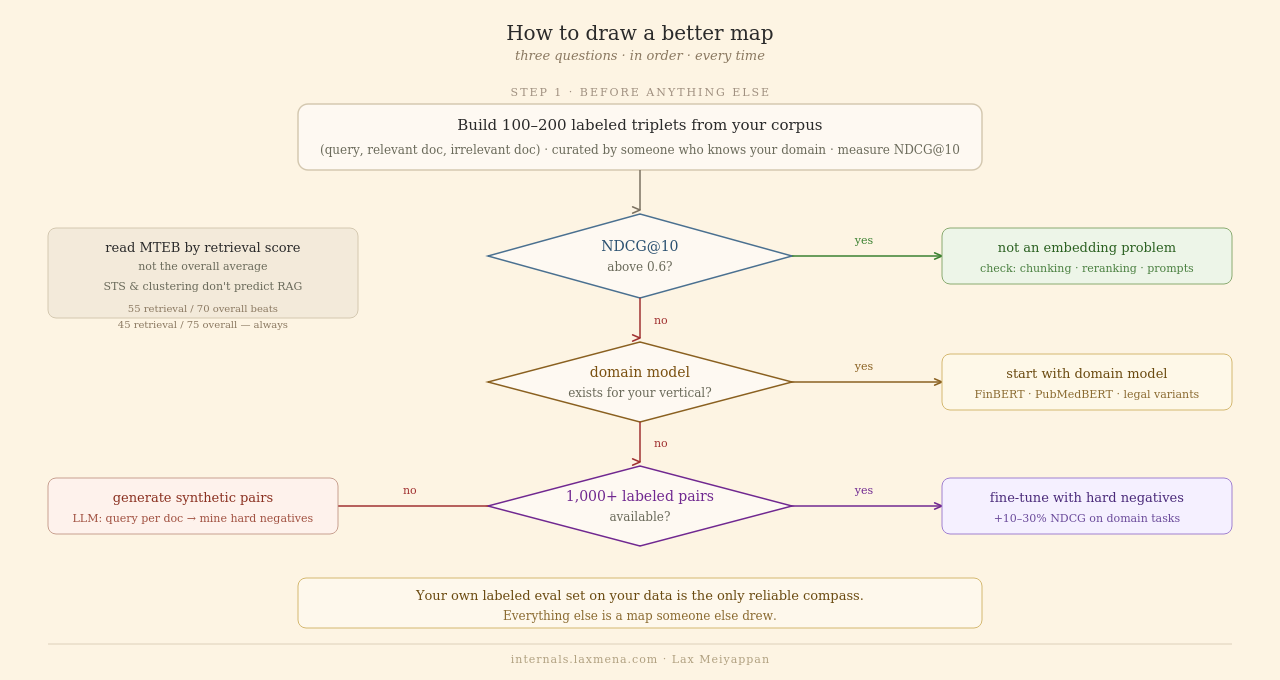
Drawing a better map
Three steps. In order. Every time.
Step one: your own labeled eval set is the only reliable compass.
Build 100 to 200 labeled triplets from your corpus: real queries, real relevant documents, real irrelevant documents, curated by someone who understands your domain. Run your current model. Measure NDCG@10. (Several python library already provides out of the box NDCG calculation).
This number is your baseline. Not MTEB. Not cosine scores. This number, on your data. If NDCG@10 is above 0.6, your embedding model probably isn’t the bottleneck. Check chunking strategy, query preprocessing, and reranking first.
If you want to automate this end-to-end rather than calculating NDCG manually, production frameworks like RAGAS allow you to programmatically compute metrics like Context Recall and Context Precision to catch these mapping failures automatically.
Step two: check if a domain-specific model exists.
For finance, biomedical, and legal: purpose-built models exist and have been empirically validated. FinBERT, PubMedBERT, legal-BERT variants. Start there and measure on your data.
For everything else: look at the MTEB retrieval sub-score specifically, not the overall average. The overall average blends in clustering and classification tasks that don’t predict RAG performance. A model that scores 55 on retrieval and 70 overall beats one scoring 45 on retrieval and 75 overall, every time.
Step three: when to fine-tune.
Fine-tune if: NDCG@10 is below 0.5, no domain model exists, and you have at least 1,000 to 5,000 (query, relevant document) pairs available.
No labeled pairs? Generate them synthetically: prompt an LLM to produce 3 to 5 realistic queries per document in your corpus, then mine hard negatives using your current embedding model. Teams using this approach on specialized domains consistently see 10 to 30% NDCG improvement.
Don’t fine-tune if: you have fewer than 500 training pairs, or your measurement says the problem is elsewhere.
One strong opinion: if your domain has heavy internal jargon, proprietary ontology, or vocabulary that means something different inside your company than it does on the web, start with fine-tuning or a domain model.
Attempting to bridge this gap purely with prompt engineering and general-purpose embeddings introduces tech-debt that scales linearly with your data complexity.
A few gotchas before you go.
High-cardinality repetitive data (think: millions of similar support tickets) makes hubness worse even after fine-tuning. The “same few documents everywhere” problem is structural when your corpus has too many near-duplicates.
Multilingual or code-heavy domains are harder than they look. A fine-tune on English financial text won’t help your Japanese runbooks or Python error traces.
And if your domain evolves fast, a startup changing its product every quarter for example, fine-tuned embeddings drift quickly. Re-training cadence and embedding versioning become a day-2 problem many teams underestimate. Weigh that cost before committing.
↓ Internals: how fine-tuning reshapes the map
Fine-tuning uses contrastive training: you give the model (query, relevant document, hard negative) triplets and train it to pull relevant pairs closer while pushing hard negatives apart.
The objective function is called InfoNCE. It frames learning as: given a query and a batch of documents, identify the correct one. The temperature parameter (τ, typically 0.05) controls how sharply the model focuses on near-misses, the documents that look like the right answer but aren’t. Low temperature = sharp focus on the hardest confusions in your corpus.
Hard negatives from your corpus are what make fine-tuning work. They teach the model the exact distinctions your users encounter, not generic web-scale distinctions. This is why in-domain hard negatives produce dramatically better results than random negatives.
The geometry side effect: contrastive training spreads vectors more uniformly across the space, reducing anisotropy. A good fine-tune with in-domain hard negatives fixes three of the four failure modes simultaneously: score compression, concept collision, and hubness.
What survives
Embedding models are coordinate systems, not reasoning engines. The map was drawn from the training corpus. It won’t redraw itself for your data.
Your cosine score measures distance on that map. A confident-looking score only tells you those two points are close together. It says nothing about whether the map covers the territory your users are asking about.
Your own labeled eval set, built from your data, is the only reliable compass. Every other decision follows from that measurement.
INTERNALS.md is a technical series on how production AI systems actually work. No tutorials. No framework evangelism. Just the layer beneath.
If this was useful, the best thing you can do is share it with one engineer who would care.
Sources
All Bark and No Bite: Rogue Dimensions in Transformer Language Models, Timkey & van Schijndel, 2021
SimCSE: Simple Contrastive Learning of Sentence Embeddings, Gao, Yao & Chen, EMNLP 2021
Understanding Contrastive Representation Learning through Alignment and Uniformity on the Hypersphere, Wang & Isola, 2020
Contrastive Representation Learning, Lilian Weng
Do We Need Domain-Specific Embedding Models?, Tang et al. (FinMTEB), 2024
Hubness Reduction Improves Sentence-BERT Semantic Spaces, 2023
Why, When and How to Fine-Tune a Custom Embedding Model, Weaviate
Hard Negative Mining, sentence-transformers documentation